TOC Analyzer Operation and calibration procedure (Schimadzu)

1.0 OBJECTIVE

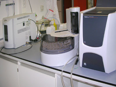
To describe a procedure for Operation and calibration of TOC analyzer (TOC – VCPH) Make: Schimadzu

2.0 SCOPE

This procedure is applicable for Operation and calibration of TOC analyzer Make: Schimadzu in company Name

3.0 RESPONSIBILITY

3.1 Microbiologist /Officer is responsible for the execution.

3.2 HOD or designee is responsible for review, effective implementation and compliance to the Operation and calibration of TOC analyzer for execution.

4.0 PROCEDURE

4.1 MATERIAL REQUIRED(UTILITIES TOTAL ORGANIC CARBON (TOC))

4.1.1 Ultra – Pure Air (CO, CO2 an Hydrocarbon shall not be more than 1 ppm)

4.1.2 High purity water (Reagent water), having TOC level shall be less than 100 ppb.

4.1.3 Stabilized power supply of 230, 50 Hz.

4.1.4 Dried clean 100 ml Volumetric flask

4.1.5 Pipette 1 ml

4.1.6 Reference standard Solution of KHP, Sucrose, 1,4 Benzoquinone

4.1.7 Micropipette with micro tips capacity 1000 µl.

4.1.8 Millipore Water

4.1.9 TOC Soft ware

4.2 Operating procedure of TOC – V CPH & OCT-1 or equivalent.(Total Organic Carbon (TOC) Analyzer Shimadzu TOC-V CPH)

4.2.1 Switching ON the Instrument.

4.2.1.1 Switch on the computer and TOC instrument.

4.2.1.2 Double click on TOC –Control V Icon on desk top.

4.2.1.3 Double click on “Sample Table Editor”. Log in ID & Password window will open. Now enter Log in ID & Password then clicks OK.

4.2.1.4 Select “New “from the File Menu or Clicking the ‘New” on tool bar.

4.2.1.5 Select the Appropriate “System” and click OK.

4.2.1.6 Give the file name for opening the Sample Table.

4.2.1.7 Now click on “connect” button on the Tool Bar Or from the Instrument Menu Select “Connect”.

4.2.1.8 Now Instrument will start initializing. Initialization Window will disappear after Auto Initializing.

4.2.1.9 Now Pressure Gauge should show 200 Kpa and flow meter should be 150 ml/min

4.2.1.10 Wait for 15 to 20 min. for getting instrument ready condition (go to back ground monitor to see back ground conditions like Furnace Temp, Dehumidifier Temp, Base line Position, Fluctuation, Noise, from the Instrument Menu).

4.2.2 Sample Measurement.

4.2.2.1 Click on Insert Menu.

4.2.2.2 Select Sample.

4.2.2.3 Sample Wizard Page 1 will open, in this page Select calibration curve button. Now browse calibration curves by selecting browse button. Calibration curve files list window will open, in this calibration list select the appropriate calibration file which is having extension of Date & Time with file name, and then click on OK.

4.2.2.4 Now click on “Next” in the 1st Page.

4.2.2.5 In the Sample Wizard Page 2, select Analysis as NPOC, and give the Sample Name & Sample ID of the Sample.

4.2.2.6 Now Click on “Next” in the 2nd Page.

4.2.2.7 In the sample wizard page 3 click on “Next”.

4.2.2.8 In the sample wizard page 4 see all the injection parameters are OK, If not select them and click “Next” (which are Shown as annexure No 1).

4.2.2.9 Now click on “Next” in the 5th Page.

4.2.2.10 Now click on “Next” in the 6th Page.

4.2.2.11 In the page 7 select “perform sample checking according to USP/EP and click on “finish”.

4.2.2.12 We can insert any No. of samples like this (from step 1 to step 11).

4.2.2.13 Now select the “start” from the Tool Bar or from the Instrument Menu. A window will be displayed in that give the vial Nos. and click on OK. After that another Window will be displayed click on “start”. Now Instrument will start analyzing the sample. To see the Peaks and Values Select “Sample window”

4.2.2.14 After completion of Analysis it will display the window of “Repeat, Next, Stop” . Select Next.

4.2.3 Creating the calibration File:

4.2.3.1 From the File Menu select “New. The new dialog box is displayed. Double click on “Calibration Curve Icon “.

4.2.3.2 Calibration curve wizard page 1. will be displayed. In this page 1 select the system and click on “next”.

4.2.3.3 in the page 2 click on “Next”.

4.2.3.4 In the page 3 select analysis as NPOC and enter the Default Sample Name and Sample ID. Also select the “Multiple Injection”. Give the Calibration File Name by Browsing and click OK. Click on “Next” on page 3.

4.2.3.5 In the page 4 select the measurement parameters and click “Next”.

4.2.3.6 In the page5 Calibration Points list is displayed. In this page click on Add and give the highest calibration point first. And give the cal points from max to min by clicking “Add” and then click “Next”.

4.2.3.7 In the page 6 Click on “Next”.

4.2.3.8 In the page 7 Click on “Next”.

4.2.3.9 In the page 8 Click on “Finish”.

4.2.3.10 Calibration file was created and now we have to insert it in the Sample Table.

4.2.4 Inserting the Calibration File in the Sample Table:

4.2.4.1 By placing cursor on the Sample Table, Click on insert menu and select Calibration Curve.

4.2.4.2 Calibration Curve File Window will be displayed, Select the Created File Name and Click on “Open” button.

4.2.4.3 Enter the Vial positions for the calibration standards directly into the vial column of the table. As the vial positions are entered in the table, they are highlighted on the tray diagram. Now click on OK button after verifying the information.

4.2.4.4 In the sample table row calibration standard was inserted.

4.2.4.5 Now click on “START” button on the Tool Bar. Again Vial position window will be displayed, click on OK, another window will be opened weather to “Keep the instrument in Running” or “Stand By” .Select “Keep Running” and click OK.

4.2.4.6 Instrument will analyze and it will give Results. For seeing Peaks, Area etc select sample window. After completing the analysis it give results.

4.2.5 For System Suitability test.

4.2.5.1 First we have to calibrate the Instrument with Zero Water (0ppb) and Sucrose (500ppb) as mentioned in above (creating the calibration File and Inserting the calibration File in the Sample Table).

4.2.5.2 After completing the calibration select “New” in the Tool Bar or from the File.

4.2.5.3 Control Sample Page 1 will be displayed, in this page select the System and click on “Next”.

4.2.5.4 In Page 2 select the “system suitability Test for USP/EP also give the file name for this control sample template, and then click on “Next”.

4.2.5.5 In page 3 Select the “Calibration Curve” and Browse for the Calibration curve. Select the cal curve and click on “open”. Click on “Next” in page 3.

4.2.5.6 In page 4 Select the analysis as NPOC, give sample Name and Sample ID as 1, 4 Benzoquinone. Then Click on “Next”.

4.2.5.7 In page 5 Set the Injection Parameters and select Multiple Injection. After that click on “Next”.

4.2.5.8 In page 6 Click on “Next”.

4.2.5.9 In page 7 Click on “Next”.

4.2.5.10 In page 8 Click on “Next”.

4.2.5.11 In page 9 Click on “Next”.

4.2.5.12 Now we have to insert the “Control Sample” sample table row.

4.2.5.13 On the Sample Table place the cursor in the row where the control sample will be inserted.

4.2.5.14 From the Insert Menu Select Control and the file name dialog box will be displayed, select the file name and click on open.

4.2.5.15 Now OCT-1 vial position window will be opened, enter the vial no and click on “OK”.

4.2.5.16 Now control sample will be inserted in the sample table row.

4.2.5.17 Now click on “Start” from the Tool Bar or from the instrument Menu.

4.2.5.18 Again OCT-1 vial position will be displayed, click on OK

4.2.5.19 Window will be displayed select on “Keep Running click OK.

4.2.5.20 Instrument will analyze sample and it will give result automatically the % of Result.

4.2.6 Procedure for Shut down the Instrument:

4.2.6.1 After completing the analysis, to shut down the instrument, Select “Stan By” by selecting Instrument Menu and by clicking “Stan by” or By clicking “Stand By on the tool bar itself. Stand By window will be displayed Select “Shut Down Instrument” and then click on “Stand By”(Instrument will turn off automatically after 30 min.) Now we can turn off the Computer by closing the Instrument Software.

4.3 Procedure for the preparation of Standard solutions and Calibration of TOC instrument:

4.3.1 4-Point Calibration:

A 4 - point Calibration curve against known standards is generated by using Potassium Hydrogen Phthalate

Identification of Potassium Hydrogen Phthalate:

Name: Potassium Hydrogen Phthalate:

Chemical Formula: C6 H4 (COOK) (COOH)

Manufacturer:

Manufacturing date:

Expiry date:

Batch No:

Packed Quantity:

Used Quantity:

4.3.2 Preparation of Standards:

Prepare known standards of 1000 ppm & 10ppm using potassium hydrogen phthalate. Prepare standards of 250, 500 and 1000 ppb using 10ppm solution through auto dilution.

Extreme precautions should be taken while preparing standards. Water required for preparation of standards is to be collected at a time to avoid contamination. Use all 100ml volumetric flasks.

4.3.3. Mother Solution:

Weigh accurately 0.2125g of KHP and dissolved in 100 ml of water It gives 1000ppm carbon concentration. This is mother solution and can be stored for further dilutions.

10ppm solution:

Take 1ml from 1000ppm solution and dilute to make a volume 100ml with zero water.

Zero ppb solution:

Zero water or blank water it self is the Zero standard. Collect it in a 100ml volumetric flask.

250ppb solution:

From 10ppm solution and set the dilution factor as 40.

500ppb solution:

From 10ppm solution and set the dilution factor as 20.

1000ppb solution:

From 10ppm solution and set the dilution factor as 10.

Generate a calibration curve using above standards and observe the linearity.

Calibration (continued):

Sample Name: KHP

Sample ID:

Oct port no:

Concentration: Zero ppb solution

Results:

Zero ppb solution:

No. of Injections Area Counts

Mean Area :

S.D Area :

C.V. Area :

Acceptance Criteria: For S.D should be less than 0.5

For C.V should be less than 3 %

Either S.D or C.V limits will be accepted.

Sample Name: KHP

Sample ID:

Oct port no:

Concentration: 250ppb solution

Results:

No. of Injections Area Counts

Mean Area :

S.D Area :

C.V. Area :

Acceptance Criteria: For S.D should be less than 0.5

For C.V should be less than 3 %

Either S.D or C.V limits will be accepted.

Calibration (continued):

Sample Name:

Sample ID:

Oct port no:

Concentration: 500 ppb solution

Results:

No. of Injections Area Counts

Mean Area :

S.D Area :

C.V. Area :

Acceptance Criteria: For S.D should be less than 0.5

For C.V should be less than 3 %

Either S.D or C.V will be the limits are accepted.

Calibration (continued):

Sample Name:

Sample ID:

Oct port no:

Concentration: 1000ppb solution

Results:

1000ppb solution:

No. of Injections Area Counts

Mean Area :

S.D Area :

C.V. Area :

Acceptance Criteria: For S.D should be less than 0.5

For C.V should be less than 3 %

Either S.D or C.V limits will be accepted.

Calibration (continued):

Results:

The linearity of the curve is observed.

S.No. Concentration Mean Area S.D. C.V.

1 0 ppb

2 250ppb

3 500 ppb

4 1000 ppb

Linearity:

Correlation coefficient:

Criterion judgment for an ideal calibration curve Correlation coefficient should be more than 0.98.

Note down the details in TOC calibration Record (Part –A) in attachment #1

4.3.4 SYSTEM SUITABILITY TEST (2-Point Calibration)

System Suitability is performed as per USP specifications.

USP reference standards or equal grade Sucrose and 1, 4 Benzoquinone are used as standards and these standard solutions are prepared once in a month.

If require Initially Peak Stabilization is performed by injecting Millipore

Standards Preparation:

Keep Sucrose in drier at 105 ºC for 2 to 3 hours.

Use pure water required for Standard preparations.

Weigh accurately 11.9mg of Sucrose and dissolve in 100ml water, to get 50ppm Carbon concentration. Use this as mother solution.

Zero ppb: Use zero water as zero ppb standard.

500 ppb Sucrose Solution: Dilute 1ml from the above mother solution with 100 ml zero water to get 500 ppb carbon concentration.

Now generate a two-point calibration curve using above standards.

System Suitability test is performed by using Sucrose and 1, 4 Benzoquinone

Identification of Sucrose:

Name:

Chemical Formula:

Manufacturer:

Manufacturing date:

Expiry date:

Batch No:

Packed Quantity:

Used Quantity:

Identification of 1, 4 Benzoquinone:

Name:

Chemical Formula:

Manufacturer:

Manufacturing date:

Expiry date:

Batch No:

Packed Quantity:

Used Quantity:

SYSTEM SUITABILITY TEST (continued):

Sample Name:

Sample ID:

Oct port no:

Concentration: Zero ppb solution

Results:

No. of Injections Area Counts

Mean Area :

S.D Area :

C.V. Area :

Acceptance Criteria: For S.D should be less than 0.5

For C.V should be less than 3 %

Either S.D or C.V limits will be accepted.

SYSTEM SUITABILITY TEST (continued):

Sample Name:

Sample ID:

Oct port no:

Concentration: 500 ppb Sucrose Solution.

Results:

No. of Injections Area Counts

Mean Area :

S.D Area :

C.V. Area :

Acceptance Criteria: For S.D should be less than 0.5

For C.V should be less than 3 %

Either S.D or C.V limits will be accepted.

6.3.5 Preparation of 1, 4 Benzoquinone Solutions:

Dissolve 7.3 mg of 1,4 Benzoquinone in 100ml water, to get 50ppm carbon concentration. Use this as mother solution.

500 ppb:

Dilute 1ml from the above mother solution with 100 ml zero water to get 500 ppb carbon concentration of 1,4 Benzoquinone

And then analyze this 500 ppb 1, 4 Benzoquinone solutions as a Sample.

Analyze the solution in NPOC method.

SYSTEM SUITABILITY TEST (continued):

Sample Name:

Sample ID:

Oct port no:

Standard Concentration: 500ppb 1, 4 Benzoquinone

Results:

No. of Injections Area Counts

Mean Area:

S.D Area :

C.V. Area :

Acceptance Criteria: For S.D should be less than 0.5

For C.V should be less than 3 %

Either S.D or C.V limits will be accepted

Results:

Concentration Area counts S.D. C.V.

0ppb

500ppb Sucrose

500ppb 1,4 Benzoquinone

Note: Prepare the standard solutions once in a month and store

at 2 to 8°C.

6.3.6 Response Efficiency:

The response efficiency (% recovery) can be calculated by the following formula.

%R = 100 [ ( Rss - Rw ) / ( Rs - Rw )]

Where Rss = Mean area counts of 1, 4 benzoquinone solution

Rs = Mean area counts of sucrose

Rw = Mean area counts of pure water

Criterion Judgment:

The system is said to be pass the test if the % recovery is in between 85% to 115%.

Note the details in TOC calibration Record (Part -B) as per the Attachment #2 format No.:IOP026/F02.

Frequency: System suitability daily and linearity for every 6 months.

4.3.7 Sample Analysis (continued):

Analysis: Analyze the samples using the latest Sucrose calibration curve & observe the results.

Sample Name:

Sample ID:

Oct port no:

Results:

No. of injections Area Concentration

Mean Area :

Mean Conc.:

S.D. Area :

C.V. Area :

Acceptance Criteria: For S.D should be less than 0.5

For C.V should be less than 3 %

Either S.D or C.V will be limits of acceptance.

4.4 Precautions (if any):

Precautions to be taken for Sample collection and Analysis:

• Use High quality glass bottles for sample collection.

• Wash the bottles with pure water.

• Prepare 2 normal Nitric acid for thoroughly washing bottles and caps.

• Wash bottles with pure water 2 to 3 times by filling to the top that is without leaving any air gap after that dry them in oven at a temperature of 110° C for 30 - 60 min.

• At sample collection point, wash glassware with sample water 3 to 4 times.

• Leave 2 to 3 liters water and then collect sample with out any air gap in the container.

• Close the cap and seal it with Para film.

• Analyze the samples immediately after they are brought to laboratory.