
Arrhenius equation
The Arrhenius
equation is the one
which explains the temperature dependence of the reaction rate
constant, and therefore, rate of a chemical reaction.
The equation was first proposed by the Dutch chemist J. H. van 't
Hoff in 1884; five
years later in 1889, the Swedish chemist Svante
Arrhenius provided a
physical justification and interpretation for it.
Common sense and chemical
intuition suggest that the higher the temperature, the faster a given chemical
reaction will proceed. Quantitatively this relationship between the rate a
reaction proceeds and its temperature is determined by the Arrhenius Equation.
At higher temperatures, the
probability that two molecules will collide is higher. This higher collision
rate results in a higher kinetic energy, which has an effect on the activation
energy of the reaction. The activation energy is the amount of energy required
to ensure that a reaction happens.

After
observing that many chemical reaction rates depended on the temperature, Arrhenius
developed this equation to characterize the temperature-dependent reactions.
The Factors
K : Chemical reaction rate and is unit of s-1(for
1st order rate constant) or M-1s-1(for 2nd
order rate constant)
A is pre-exponential
factor or
frequency factor and is realted to mollecular collisions Deals
with the frequency of molecules that collide in the correct orientation and
with enough energy to initiate a reaction. It is a factor that is determined
experimentally, as it varies with different reactions.In
unit of Lmol-1s-1 or M-1s-1(for 2nd order rate constant) and s-1(for
1st order rate constant. Because frequency factor A is related
to molecular collision, it is temperature dependent. Hard to
extrapolate pre-exponential factor because lnk is only linear
over a narrow range of temperature
Ea: The activation energy is the threshold energy that the
reactant(s) must acquire before reaching the transition state. Once in the
transition state, the reaction can go in the forward direction towards
product(s), or in the opposite direction towards reactant(s).A reaction with a
large activation energy requires much more energy to reach the transition
state.Likewise, a reaction with a small activation energy doesn't require as
much energy to reach the transition state. In unit of kJ/mol. -Ea/RT resembles
the Boltzmann distribution law.
R: The gas constant. Its value is 8.314 J/mol K.
T: The
absolute temperature in which the reaction
takes place. In units of Kelvin (K).
Application of Arrhenius equation
Application of the Arrhenius equation in
pharmaceutical stability testing is straightforward. In the isothermal method,
the system to be investigated is stored under several high temperatures with
all other condi- tions fixed. Excess
thermal exposure accelerates the degradation and thus allows the rate constants
to be determined in a shorter time period.
Most accelerated testing models are based on
the Arrhenius equation
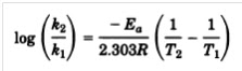
where k2 and k1 are rate
constants at temperature T2 and T1, respectively; Ea is
the activation energy; and R is the gas constant. Temperature is
in kelvins.
This equation describes the relationship
between storage temperature and degradation rate. Use of the Arrhenius equation
permits a projection of stability from the degradation rates observed at high
temperatures.
Activation energy, the independent variable
in the equation, is equal to the energy barrier that must be exceeded for the
degradation reaction to occur. When the activation energy is known (or
assumed), the degradation rate at low temperatures may be projected from those
observed at “stress” temperatures.
The relationship between drug concentration
[D]after time (t) for a first-order equation is
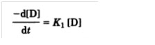
where K1 is the reaction rate
constant at a given temperature. Integrating from t = 0 to t =
t, one obtains
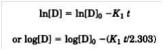
where [D]0 is the drug
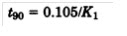
concentration at time 0. By substituting 0.90 [D]0 = [D]0
in the equation above, the time required to reach 90% of the original
drug concentration can be shown to be
A common practice of
manufacturers in pharmaceutical and diagnostic reagent industries is to utilize
various shortcuts, e.g., bracket tables and the Q rule, to
estimate product shelf life. These techniques (see below) share the advantage
that decisions may be made by analyzing only a few stressed samples.
However, they are based on
assumptions about the activation energy of product components and are valid
only in so far as these assumptions are accurate. Whatever method is chosen,
the validity of product stability projections depends on analytical precision,
the use of appropriate controls within the experimental design, the assumptions
embodied in the mathematical model, and the assumed or measured activation
energy of product components.
Reaction rate is influenced by
pH, tonicity, the presence of stabilizers, and so forth. Key product component(
s) may degrade (or otherwise become unavailable) through multiple mechanisms .
In complex chemical systems, therefore, minor variation in formulation can
profoundly affect lot-to-lot stability and, indeed, the activation energy of
product degradation. Consequently, shelf life projected from accelerated
studies must be validated by appropriate real-time stability testing.
Rapid
Techniques for Projecting Shelf Life
Examples of shortcuts for projecting product
shelf life for storage at 5 #{1i7n6c}lCude the QRule and bracket table methods.
QRule.
The Q Rule states that a product
degradation rate decreases by a constant factor (Q10) when the
storage temperature is lowered by 100C. value of Q10 is
typically set at either 2, 3, or 4 because these correspond to reasonable
activation energies. For larger shifts in temperature, the rate constant
changes exponentially with temperature, and is proportionalt (Q10)n where n
equals the temperature change (0C) divided by 10. For example,
the estimated decrease in degradation rate caused by lowering the storage temperature
by 50 0C(Q10)5 because n = 50/10 = 5
(see Table 1). This model falsely assumes that the value of Q does not
vary with temperature. A more detailed treatment has been published.
A Q10 value of
2 provides a conservative estimate, and results calculated with this value are
considered probable. A Q10 value of 4 is less
conservative and yields results considered tobe possible. To illustrate
the application of the Q Rule in predicting shelf life, assume that 90%
of phencyclidine (PCP) is recovered after 26 days at 550C. stability
of PCP under refrigerated (50C)
conditions may be estimated [26 days/(Q10)5] as follows:
(a) PCP is probably stable
for 832 days (2.3 years) if Q10= 2.
(b) PCP may be stable
for 6318 days (17 years) if = 3.
(c) PCP is possibly
stable for 26 624 days (73 years) if Q10 = 4.
Table
1 : Q10 Factors
|
||
Q10
|
Ea [Kcal/Mol]
|
(Q10)5 = Q50
|
2.0
|
12.2
|
32
|
3.0
|
19.4
|
243
|
4.0
|
24.5
|
1024
|
Bracket tables.
The bracket table technique
assumes that, for a given analyte, the activation energy is between
two limits,e.g.,between 10 and
20 kcal. As a result, a table may be constructed showing “days of stress” at
various stress temperatures. The use of a 10 to 20 kcal bracket table is
reasonable, because broad experience indicates that most analytes and reagents
of interest in pharmaceutical and clinical laboratories have activation
energies in this range .

Because the bracket table
provided in Table 2 does not specify stability requirements at a stress
temperature of 550C, conservative use of the table requires that
projections be taken from the 47.50C. The PCP stability assumed in
the Q Rule illustration (26 days) exceeds the six-month stability
requirement (16.6 days) for the 10 kcal model. Thus, the interpretation of the
bracket table is that PCP is probably stable at 50Cat least
six months. Furthermore, because the assumed 26 days also exceeds the nine days
stability required for the three-year 20 kcal model, it is possible that
PCP is stable for at least three years.
Prudent use of either of these rapid
techniques would dictate that data at three or four higher temperatures be incorporated
into the projection of refrigerated shelf life. To evaluate the usefulness of
the Q Rule and the bracket table in this example, one must determine the
activation energy for PCP and then project the refrigerated shelf life by using
the Arrhenius equation.


.JPG)


![Difference between Stability[Shelf life] Specification and Release Specification](https://4.bp.blogspot.com/-O3EpVMWcoKw/WxY6-6I4--I/AAAAAAAAB2s/KzC0FqUQtkMdw7VzT6oOR_8vbZO6EJc-ACK4BGAYYCw/w680/nth.png)
0 Comments